Newsletter List


Newsletter Issue #75, January 2005

ICAP/4 Consumer is Here!

Welcome to ICAP/4 Consumer! This is Intusoft’s analog and mixed-signal simulation offering for the consumer marketplace, soon available through Fry’s Electronics and orderable directly through Intusoft. The software furnishes many of the features of the ICAP/4 Rx offering, less capability such as in-depth interactive modification of components and multiple schematic configurations. Design size is limited to around 100 components and features 3,000+ simulation models of a variety of parts. Its parts browser, simulation, and waveform viewing are all easy to use, as with all ICAP/4 packages. A New User’s tutorial gets you up and running in minutes. Combined with a more extensive operation manual, it’s all that’s needed to tackle many types of electronic design. ICAP/4 Consumer is ideal for the hobbyist, student, electronic professional, adult education instructor, engineer, and science fair enthusiast. ICAP/4 Consumer retails for $249.

In This Issue
1
1

ICAP/4 8x11 is Released

2
3

The Encoder Model

6

Designing the Decoder

9
10 Counting the Pulses and Displaying the Results
11 Tesla Coil Project
20 Tips for Faster Design

ICAP/4 8x11 is Released

"Intusoft released its 8.x.11 software for the ICAP/4 analog, mixed-signal and mixed-systems SPICE simulation tool suite on October 13th, 2004. 8.x.11 adds to its previous 8.x.10 success by providing several operability enhancements for design entry, simulation and design verification. Two new convergence algorithms, ICSTEP and GEQFREQ, are an integral part of 8.x.11, primarily targeted for design involving feedback using cascaded high-gain amplifiers. ICSTEP has also been an integral aspect in the creation and simulation of complex custom IC models.


Intusoft’s new custom modeling service has provided more than 650 new component models as part of 8.x.11, while its simulation R,L,C component database has been augmented by several thousand new parts. The database was driven by an intensive effort to assign a gamut of footprint properties for these parts. The wealth of electrical and mechanical properties derives from NASA standard, ultimately for the export from ICAP/4’s SpiceNet design entry system to Bartels’ AutoEngineer PCB software. This is now available in 8.x.11 and the ICAP/4 demo disc.


Freehand artwork capability was added to SpiceNet, along with enhanced help and documentation. The ability to choose schematic or waveform-viewing environments as active after a simulation, conserves time over repetitive debug cycles, particularly when combined with any of three modes for instantly updating existing waveforms in IntuScope. New advanced signal processing functions were added to IntuScope’s collection of 125. Added capability was also created for managing design projects, while ICAP/4’s component Library Manager was placed into all non-ICAP/4Rx packages. Intusoft’s new IBIS2SPICE Converter supports IBIS models through version 3.2, and is part of all non-ICAP/4 Rx ICAP/4 software.


Make sure you are current with maintenance or you’ll miss out on all the new features and functionality in 8.x.11. Special discounting is available to those whose maintenance has elapsed for more than a year.

TOP

Turns Counter Project

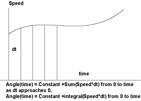
An electronic circuit will be constructed using the ICAP/4 package that counts the turns of a rotating shaft. Counting shaft revolutions is a common problem. From a car odometer to a model robot, the problem is frequented in many real-world instances.


Of course, we need to know about pi to change a rotational speed, which we will simulate using ICAP/4 in revolutions per minute (RPM), and into an angle that changes with time.


First, a definition of the angular unit is needed. Degrees are used in everyday conversation, however, as a dimensionless quantity, the radian makes more sense in mathematics and engineering. Specifically, an angle A sweeps out a segment of a circle. The segment length (s) is given by s = r*A. Then A = s/r radians. When s=C, A=2*pi, so there are 2*pi radians in a circle or:


2*pi radians = 360 degrees.


Finally RPM is converted to radians/second as follows:


Angular speed=RPM*2*pi radians/revolution*60Second/minute*time=pi/30*RPM rad/sec


Next, the angle must be computed. For constant RPM, just multiply by time. However, if RPM is allowed to vary with time, we need to sum each RPM*dt, where dt is an arbitrarily small time interval, as shown in Figure 1. As the time interval dt approaches 0, the function is defined as the integral.

Figure 1: When Speed varies with time, it is necessary to integrate Speed to get the proper angle.

Fortunately, you don’t need to do any work to get the sine/cosine functions because there is already a model in the ICAP/4 library that does all the work for you. It’s called Voltage Controlled Oscillator (VCO), and it performs integration using a built-in Laplace function. The sine/cosine functions are made with behavioral elements. The model is described in detail in http://www.intusoft.com/nlhtm/nl67.htm#costas. The application for that Newsletter (link) was a 900 MegHz communications receiver. Here, the same model is used but with frequencies below 1Hz!

TOP

The Encoder Model

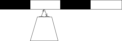
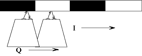
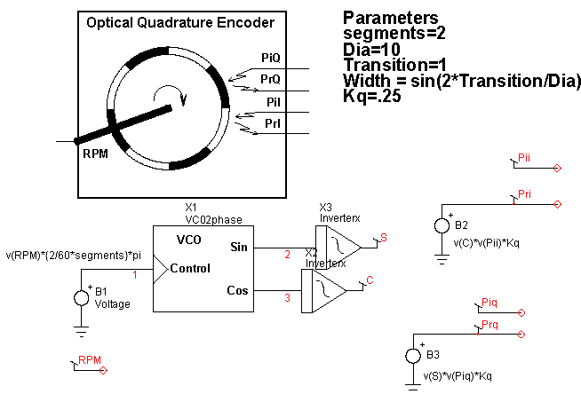
Marking the shaft with an alternating black and white pattern, shown in Figure 2, allows an optical photo sensor to monitor shaft rotation.

Figure 2: A simple optically readable pattern

However, if the rotation direction is also needed, another sensor is usually added. Another pattern can also be added. The new pattern shown below (Figure 3) has the black and white stripes staggered. This arrangement is known as quadrature coding. If motion I is in the “forward” direction, then a 0-1 (black-white) transition in the “I” channel when the Q channel is false (black) is counted as a clockwise revolution. Conversely, a 1-0 transition counts as a counter-clockwise revolution. The logic reverses based on the quadrature channel so you can get 2 pulses for 1 pattern cycle.

Figure 3: Adding a second pattern and sensor let’s you count rotation in 2 directions.

Another way of building the quadrature signals is to stagger the sensors along a single pattern as shown in Figure 4. If half the shaft is painted white and the other half is painted black, separating the sensors by 90 degrees gives the desired result. The 90-degree separation places one of the signals in quadrature with the other.

Figure 4: Staggering the sensors along a single pattern also works.

For shafts that are rotating the radial distance from the center of the shaft is given by r = x^2 + y^2. At an angle, A, y = r*sin(A) and x=r*cos(A). But with A, the shaft angle changes with respect to time. For a constant RPM, A increases with time just like the distance you drive at a constant speed. But the speed can increase or decrease, so you must integrate speed to obtain the correct angle. The VCO model is used to integrate the speed input and get the sine/cosine signals. The reflected optical signal has a cosine-tapered waveform because the illumination is a disc shaped light beam. As the pattern passes across the illuminating disc, the reflected light gradually changes from one state to the other with a cosine-like shape. The disc gets larger as the distance between the sensor and target pattern is increased and the spatial rise-time increases. If the light beam disc diameter is known along with the shaft diameter, then the spatial “rise-time” of the reflected signal can be calculated as follows:

Let Arise = angular rise “time”
DI = incident illumination diameter
DS=shaft diameter
Arise = DI / (pi*DS)

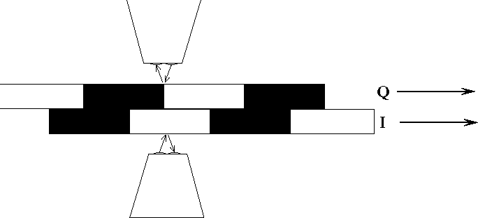
Now it is possible to have the pattern repeat in order to increase resolution. Yet, Arise is unaffected. But Arise will set an upper limit on the number of times the pattern can be repeated. Putting it all together in Figure 5.

Figure 5: The complete encoder model and its symbol.

The ICAP/4 library models for VCO and inverterx do exactly what is needed. VCO was developed for communications modulation and demodulation, while inverterx was made as a soft transition cosine shape limiter. The parameters passed into the model are:


Width: sets the transition behavior in inverterx.
Segments: sum of black and white bands to account for more pattern repetitions.
Kq: the reflection coefficient: If desired, you can sum noise, such as 120Hz signals from nearby incandescent and fluorescent lights. It’s best if you shield the photo micro sensor from this source of noise. The one used here has an infrared filter to help eliminate visible light interference.
Dia: the encoder diameter (any units)
Transition: the distance between on-off detection (same units as Dia)

TOP

Designing the Decoder

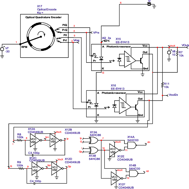
So far, the project design has focused on getting an electro-optical interface that can act as a signal generator to test the project design. From the beginning, the I and Q signals are modeled with slow rise-times. Something must be done to sharpen these rise-times so they can be used as the clock for an up/down counter. Reviewing the available optical reflection sensors, there are some that have hysteresis limiters built-in. Hysteresis is a form of positive feedback that sharpens rise-times. The OMRON EE-SY413 is one such device. It was modeled using a previously developed opto-isolator with its optical path broken to output incident light and receive reflected light. Its current transfer ratio (CTR) was adjusted based on manufacturers data. Hysteresis was added using a SPICE3 behavioral switch. Initially it wasn’t known if the rise-time of the device was as fast as required, but it was tested in the lab and found adequate for use as a clock for CMOS devices. It’s now an ICAP/4 library item.


Next, the up/down counting logic needs to be designed. It’s first necessary to know the current I and Q states, along with the previous states (called Ip and Qp). The reason behind this is to be able to detect a change in rotation direction soon after an up/down transition is made. These previous states are measured using delay multi-vibrator (DMV) constructed using CMOS inverters. The DMV uses positive feedback to make sharp transitions. These DMV transitions will form the active clock edge, which is the transition where the synchronous logic states are examined. The I, Ip, Q and Qp states can be drawn in a logic truth table, shown in Figure 6. To make the truth table, take the I signal with its pattern of 0110. This pattern will repeat at the rotation frequency (RPM). Then, Ip is the previous pattern, 0011. Similarly you can enter the Q and Qp parts of the table. Next, reverse the rotation direction and make the second truth table.

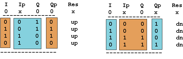
Figure 6: Logic states for cw and ccw rotation.

The logic states have been shaded to show groupings that are useful. The cyan colored groups represent “exclusive or” patterns, while the brown shade shows “exclusive or not” groupings. By inspection we can write:


up = (I xor Qp)n &(Ip xor Q) and dn = (I xor Qp) & (Ip xor Q)n

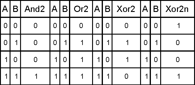
There are three basic Boolean operations. In engineering they are called AND, OR and NOT. Mathematicians call them intersection, union and negation, and use symbols that aren’t on your keyboard to represent them. Sticking with engineering notation, we’ll define the following operations:

AND &
OR +
NOT n

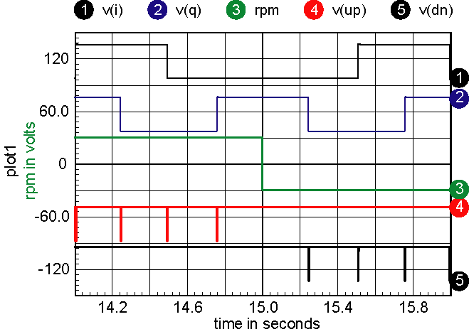
The exclusive or is encountered frequently enough to deserve its own operator; we’ll use xor.


A truth table is a table of all interesting states and a corresponding result. A logic equation expresses the results as illustrated in the table below for some two-input results.

Table 1: Results for two input combinations

And2 = A & B = (An + Bn)n
Or2 = A + B = (An & Bn)n
Xor2 = An & B + A & Bn = (An&Bn + A&B)n
Xor2n = (An&Bn + A&B) = (An & B + A & Bn)n
Notice that A&B+A&D = A&(B + D) so that OR follows algebraic rules for addition and AND follows algebraic rules for multiplication. The completed decoder circuit is shown below in Figure 7.

Figure 7: The complete decoder using the encoder model for testing.

Figure 8: The up/down counting pulses with a rotation reversal at 15 seconds.

The up/down pulse widths are very short, so to see then using an oscilloscope, you must trigger on one of the I or Q signal edges and expand the trace to 100 microseconds.

TOP

Exclusive OR, Where Analog Meets Digital

Before moving on to the up/down counter and display circuitry, let’s make a side trip to see how the technology that’s been used here applies to several other applications. The exclusive OR is the basis for digital addition. It’s fundamentally the sum of two bits. But from an analog perspective, if you let a logic “one” be defined as +1, and a logic “zero” as –1, then the exclusive OR is actually the product of the inputs. Using that property, taking two signals that are at the same frequency, but phase shifted, like the I and Q signals in the decoder, then the average value of the exclusive OR is proportional to the phase shift. That means that an analog phase detector can be formed using an exclusive OR and filtering the output with a low pass filter to get phase. When the signal to noise ratio is fairly high in a communications channel, you can limit the signal, turning it into a binary data stream. Then, an exclusive OR can be used to detect phase or frequency encoded signals. Of course, you don’t really need +1 and –1 for logic levels, but using this thought process simplifies the math. Using CMOS for the logic is advantageous because the logic one and zero values are at the power supply rails, providing analog accuracy.


Looking further, suppose we want to use a laser to measure distance or speed. We can construct a Michelson Interferometer and place I and Q sensors ¼ wave apart on the fringe pattern. If the light wavelength is 1 micron (10^-6 meters), then you would obtain a 4 MegHz signal for a 1 meter/second velocity. The same thing can be done with radio waves or sound waves. The table below shows the sensitivity for 3 cases.

  Wavelength Frequency Sensitivity
  V/F V/L to 1 m/sec velocity
Optical 1u 3e14 4 megHz
Radio .2 1.5g 20 Hz
Sound .01 30 kHz 400 Hz

Table 2: Sensitivity

Note: For radio and optical applications c = 3*10^8 meters/second, for sound in the atmosphere, c is about 300m/sec (lots of pressure and temperature variation).

The optical detector is extremely sensitive and is being used by LIGO, the Laser Interferometer Gravitational Wave Observatory. Similarly, a fiber-optic coil can be used to detect vibration and/or rotation, making a sensitive microphone of a gyroscopic rotation sensor. The technique can be used to measure position from a GPS signal with accuracy on the order of 2cm (1/25th of a wavelength). Acoustic applications include ultrasound and sonar systems.

Some very simple equations blossom into an astonishing array of applications. Taking the math one step further leads to 3d-imaging systems and hologram construction; but that’s for another time.

TOP

Counting the Pulses and Displaying the Results

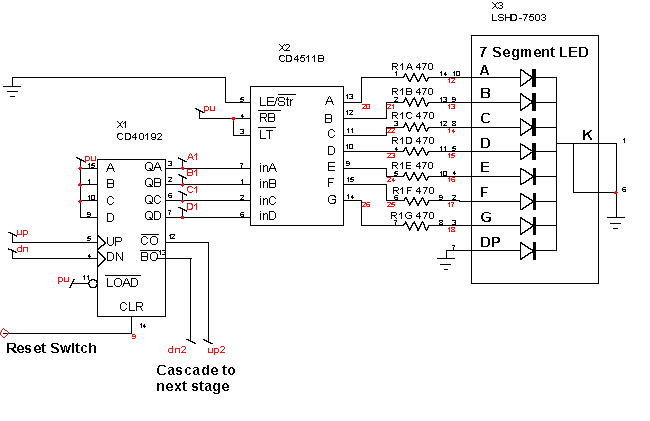
To complete the project, the up/down pulses need to be counted and displayed. For an inexpensive stand-alone application it was decided to use CMOS logic. Alternatively, you could interface directly with your computer using a PIC (Programmable IC) connected to a USB port. A CD40192 Binary Coded Decimal (BCD) up/down counter accumulates 10 pulses per stage. It easily cascades to get the count as large as you want; our design used three stages to accumulate up to 1000 quarter turns. The BCD output is displayed by first decoding each digit to drive a 7 segment display. The seven-segment display is a LITEON LSHD-7503. It’s connected to the CD4511B Decoder using 470 ohm resistors that can be purchased in a 16 pin Dual in-line package (DIP). The parts can be interconnect using a Printed Wiring Board (PWB), soldering or wire wrapping. If you use a PWB, your probably want to use the Small Outline IC (SOIC) packages otherwise DIP packages are easier to work with.

Figure 9: One of 3 stages of the counter and readout display

TOP
Tesla Coil Project

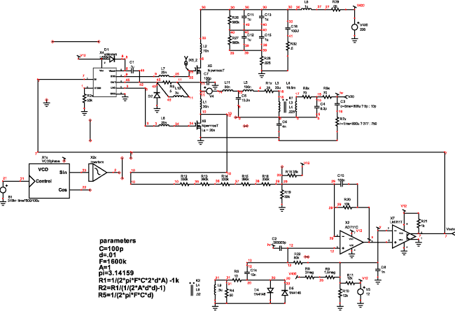
Construction of Tesla Coils is described in a variety of ways on the Internet. What’s in common is a large diameter coil with a very large step-up turns ratio. Nicoli Tesla, who invented the Tesla Coil, used the breakdown of a spark gap to drive the primary. However, modern power electronics give us a much better set of analysis tools and hardware components to couple energy more efficiently into the coil.


Starting with a 10-inch coil wound on a 3.5 in. diameter form using #30 wire, a circuit model was constructed.


Winding notes: The secondary was wound on a 3.5in OD PVC pipe, using 4 stripes of 1.5 mil double stick tape to hold the wire in place as it was wound. End caps were used to support the coil vertically. The coil was wound by hand with the coil in the vertical position. The feed wire spool was placed on a CD bobbin that was taped to a desk so it was free to rotate as we wound the coil


Laboratory measurements were made to find the coil self-inductance and resonant frequency. An inexpensive LC meter measured the inductance, and a signal generator was used to excite the coil at its self-resonant frequency as shown in Figure 10.

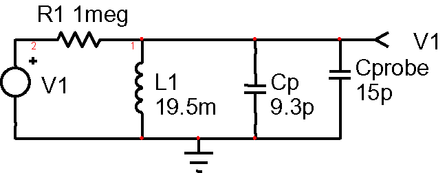
Figure 10: Resonance measure at 228.9kHz, loaded with a 15pf scope probe, leaves 9.3p for the actual coil.

Interestingly, the resonance without the scope probe is 373kHz, which is a period of 2.67u. That’s very close to 4 times the propagation delay of the coil (900 turns * pi * 3.5 1n /12in = .824u). So we could calculate Cp=1/(L*(2*pi/(4*Td))^2. Using that method, we get 14pf.


Next, a test primary was wound and its coupling coefficient and self-inductance were measured. The first test used 2 turns of wire for the primary. The coupling coefficient was so low that it couldn’t be measured. Next we wound 10 turns near the bottom of the primary and measured a coupling coefficient of 0.225


The resulting model is shown in Figure 11.

Figure 11: The equivalent circuit of the Tesla coil and its primary using SPICE coupled inductors.

The method of constructing the primary must now be considered. The primary needs to use larger wire (smaller AWG) than the secondary. This is because the current is larger in the primary, and the power loss is proportional to the current squared times the resistance. Unfortunately, at higher frequencies, current tends to flow on the outside region of the conductor; this is known as the skin affect. You can use Intusoft’s demo Magnetics Designer software to find the AC resistance of various wire sizes vs. frequency.


Past the skin depth mentioned above, only 1/e of the total current is found. For #30 wire at 400kHz, the Ratio of AC to DC resistance is 1.68. The DC resistance was found to be 85 ohms using a digital multimeter. The secondary AC resistance is then 1.68 * 85 = 142.

Winding the primary: Multiple strands of #30 were used for the primary. This wire is called Litz wire. The idea is to braid each wire strand randomly through the Litz bundle to prevent the magnetic field from moving the current to the outer surface. You can buy Litz wire or make your own. To make your own from #30 wire, you first need to twist several strands together. We used 4 stands for that purpose. Then, take the twisted wire bundles and twist them together to form the Litz wire. We used 3 bundles for a total of 12 conductors. The total DC resistance was measured as .15 ohms, and would be .25 Ohms at 400kHz. To twist the wire, first measure out about 10% more than the length you need. Anchor the four parallel strands on a tripod and connect the other end to an electric drill or lathe. Then, wind about 10-20 turns per foot. Combine the finished bundles, twisting them about 5-10 turns per foot. Wind the Litz wire onto a wire dispenser. Be careful to make sure it doesn’t twist. #30 wire is fairly forgiving. It’s strong enough to resist breaking and it can be stripped by burning the insulation and sanding the charred insulation with fine sandpaper. You can buy wire with basically 2 kinds of insulation: Formvar or enamel. The Formvar insulation is copper colored. It cannot be soldered. It must be stripped as described, or etched using chemicals, or by scraping the large wires. The enamel insulation, sometimes called solder-eze, is usually colored red or green and can be soldered without stripping; a combination of heat and pressure destroys the insulation. Before winding the primary, you must provide the insulation necessary to prevent arcing. We used 20 mils of polyurethane tape, followed by 0.1in of double stick tape. The double stick tape holds the primary in place while you wind it. The primary must be wound over the bottom of the secondary to minimize the primary-secondary voltage stress.

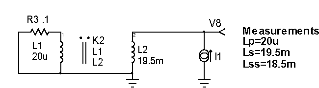
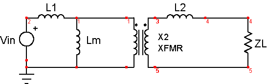
The self-inductance of the primary and secondary was measured using an inexpensive LCR meter. The coupling coefficient was calculated by shorting the primary and measuring the secondary inductance. SPICE has built-in models for coupled inductors. It requires the open circuit inductance value for each winding, plus a coupling coefficient that’s greater than 0 and less than 1. Simulations were run with the primary shorted, varying k (the coupling coefficient) until the simulation agreed with the measurement. Notice how simulation replaced development of algebraic equations.


Another way of looking at the transformer model is by using a Y network of inductors and an ideal transformer to account for the turn’s ratio. That’s the model most frequently used in power electronics because of its close relationship to the physical device.


For power electronics, the coupling coefficient is usually so high that the leakage inductors (Le) coupling the energy is small compared to the self-inductance (Lm). When that is true, the Leakage inductors are calculated as (1-K)*Lm. The inductors can be moved through the magnetizing inductance to either side of the transformer, thereby eliminating one of the inductors. Figure 12 below illustrates this paradigm.

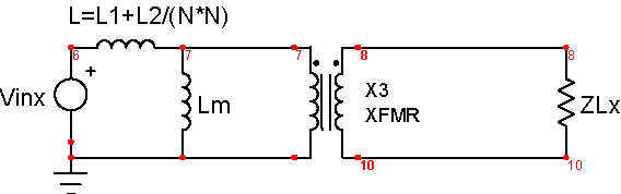
If Lm >> (L1 + L2/(N*N)), then the following preserves the open and short circuit simplification properties

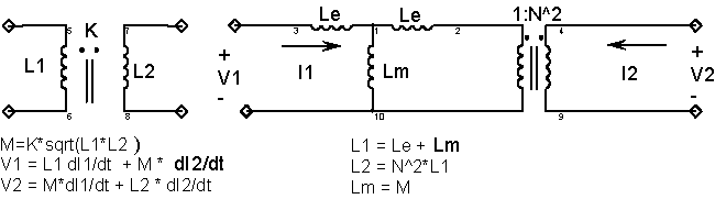
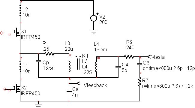
Figure 12

However, this is not the case for the Tesla Coil. Figure 13 shows the Y model. Unfortunately the math results in a negative inductance and the physical insight is lost in the mathematics.

Figure 13: The SPICE coupled inductor and its equivalent circuit: Lm = 140u, Le=- 120u, N=31.2

Because the coupling coefficient is so low, the primary self-inductance tends to short out the driving signal. However, if a series/parallel set of capacitors is used to couple energy, then the input impedance will increase at resonance, thus achieving decent power transfer efficiency. The LCC configuration shown in Figure 14 was chosen to match the Tesla Coil impedance with the half-bridge power capability. The bridge transistors can switch 14 amps at 400 Volts. If the design is setup to output around 250 watts with a 200 Volt input, then an extra boost converter can double the voltage and multiply the power by 4.

Figure 14: The complete Tesla Coil Model with the circuitry using Cp and Cs to couple energy from V2 to Vtesla.

If Cp+Cs is made constant, the smaller values of Cs will reduce the required input current, but increase the voltage. That’s how the Tesla Coil is matched to the half bridge capability. When Cs+Cp is reduced, the voltage at Vfeedback will increase and cause greater stress on the capacitors.


If Vtesla is sufficiently large, the air breaks down and plasma streamers will form. The fields near the Tesla Coil can be increased by making geometric discontinuities in the Tesla Coil “antenna.” A pair of pyramid shaped cooking molds were used for this purpose. The plasma will increase the capacitance and add series resistance to the circuit. That affect was simulated by switching the load capacitance and resistance.

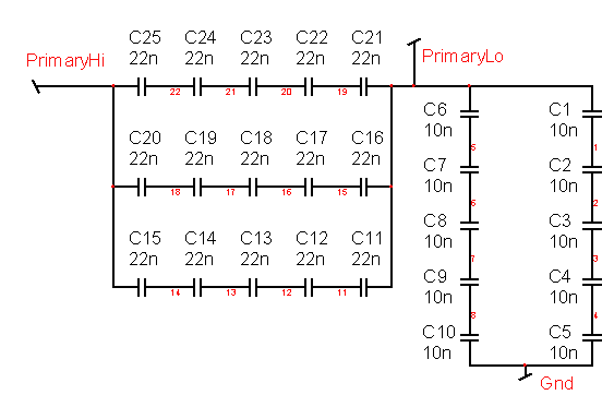
Cs was formed using 10, 10nf polypropylene capacitors: 2 parallel banks of 5 in series. Cp was formed using 15, 22nf polypropylene capacitors: 3 parallel banks of 5 in series. That furnishes a primary RMS current capability of 2.8 amps; that’s less than the MOSFET capability, so it will be necessary to limit operational time to avoid over heating.


The MOSFET switches can be made to switch on and off with virtually zero transient stress. This is accomplished by adjusting the current phase with respect to the switching voltage. The tuned circuit needs to operate above its resonant frequency for the LCC configuration used. Table 3 shows the simulation results for several values of capacitance with a 100Vac input.

CP
kv/amppk@100vdc
freq
maxvrms
operating point
6.2n
.958
373k
19k
v = 80, ipk = 20
8.8n
1.79
344k
35.8k
v = 160, ipk = 20
13.2n
4.16
321k
72.9k
v = 400, ipk = 17.4
17.6n
7.19
313k
54k
v = 400, ipk = 7.7

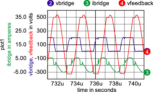
Table 3: Trading off capacitor values verses stress and performance

When operating at the proper frequency, the parallel capacitor eliminates inductive spikes when the transistors turn off. Figure 17 illustrates this using the third case in Table 3. The trick is to adjust the resonant current phase such that the voltage will switch to the opposite power rail when the current is turned off. Then, the voltage across the opposite MOSFET will be zero when the other transistor switches ON. These values allow IRFP450 MOSFETS to operate at about 400 VDC input while delivering 1kw. Cs and Cp are selected to stress the capacitor and MOSFETS to their limits at the highest input voltage.


The current in Cp will be (Cp+Cs)/Cs times the current in Cs. These are very high currents and require special capacitors to withstand the stress for continuous operation. Spark-gap driven Tesla Coils operate on a very small duty ratio. If we do the same, for example running the coil for 1ms at 120Hz, the stress can be reduced by 1/8. If polypropylene capacitors are used, a series-parallel bank can be made as shown below in Figure 15. Another choice is making one yourself, or using Mica capacitors that are very expensive (we were quoted each $150 for 1nf 3kv 2.4Amp @ 300kHz). Connecting 5 10nf polypropylene capacitors in series results in a 2nf capacitor that can carry 1.2 amps continuous current. That comes to 2.4Amps for the 4nf capacitor. Similarly, the 13nf capacitor is made from series-parallel combinations of 22nf capacitors. The current limit is based on power dissipation, P = I*I*R. If the power is pulsed ON for a duty ratio, D, then the average dissipation is D*P. Therefore we can increase the I*I product by 1/D. To go from 2.4 Amps to 6.5 amps, the I*I ratio is (6.5/2.4)^2 and D= (2.4/6.5)^2 = .136. That results in just over 1ms at 120 Hz rep rate. The final capacitor bank is shown in Figure 15.

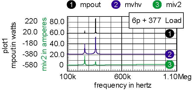
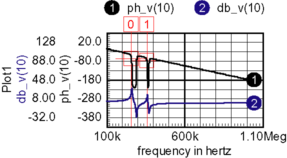
Figure 15: Connecting capacitors in series-parallel combination gets the desired current and voltage rating.

Figure 16: This shows the load current and half bridge output when the drive frequency is 363.956kHz, Cs=4n, Cp=13n.

The tesla coil can be operated at one of 2 resonant frequencies. Figure 17 shows the small-signal transfer function of the Tesla Coil.

Figure 17: The Tesla Coil exhibits 2 resonant frequencies, the second being preferred.

mpout is the magnitude of the power delivered to the load
mvhv is the magnitude of the Tesla Coil output voltage
miv2 is the magnitude of the bridge current

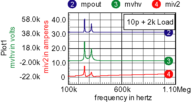
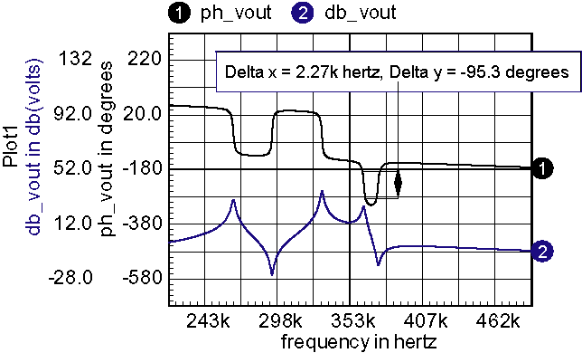
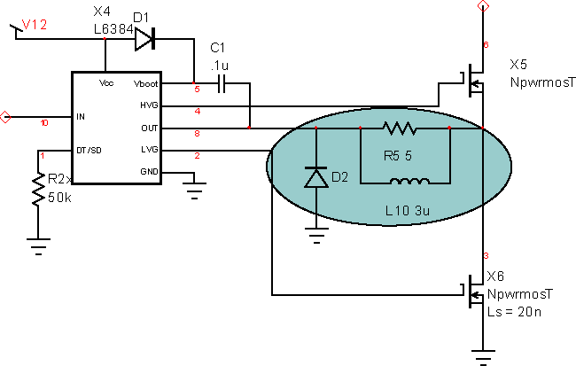
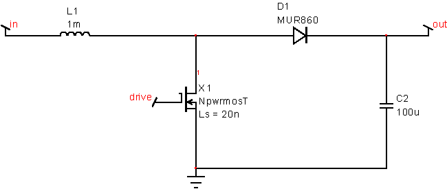
When the Tesla Coil starts up, the voltage increases until plasma streamers form. These streamers extend the effective area of the load capacitor, increasing its capacitance and at the same time dissipating power. The small signal transfer function is shown in Figure 18 for a simulated plasma discharge.

Figure 18: Plasma discharge lowers the second resonant frequency; either frequency produces an acceptable operating point.

The small-signal transfer function of the half bridge circuit and its driver are shown in Figure 19. The half bridge driver has a .5usec delay. Part of that delay is used keep both drivers off during switching transitions. It eliminates power shoot-through caused by having both the upper and lower driver turned on at the same time. The delay is simulated using a transmission line to get the transfer function using an AC analysis.

Figure 19: Small signal transfer function is shaped for self-oscillation at either resonant frequency by reversing the feedback polarity.

A self-oscillation situation occurs when there is positive feedback at the oscillation frequency, and negative feedback at DC to stabilize the operating point. It turns out that either of the resonant frequencies can be selected by coupling some of the output voltage back into the circuits input. Reversing the feedback polarity selects one of the resonant peaks.

Figure 20: The Bode plot shows that the self-oscillation frequency can be adjusted over a 95-degree range by adding phase lead.

Finally, the compensation is designed using op-amps. The feedback signal is limited using diodes to keep the op-amps within their specified operating region.

Figure 21: Compensation for self-oscillation using op-amps

Driving the half-bridge: The resonant current results in a reverse current polarity in the half-bridge transistors of Figure 22 below. The negative voltage increases the driver boost voltage and can damage the driver if negative voltage is lower than -5 volts. This condition is prevented by using a clamping circuit at the driver output. Several windings on a small MPP core yield the desired resistance (core loss provides the resistance). Alternatively, you could use a non-inductive resistor. You can re-wire it to connect the sweep generator to the input to see what happens as the drive frequency changes.

Figure 22: Half-bridge driver output needs to be clamped to prevent excessive boost voltage.

Increasing the voltage: The tesla coil needs up to 400 volts, but the off-line rectifier barely produces 200 volts. To get the increased voltage, a boost regulator is needed as shown in Figure 23.

Figure 23: A simple unregulated boost circuit increases the output.

The boost converter has the following in-out relationship if the inductor always conducts current.


Vout = Vin/(1-Don).


The circuit can be driven from a simple timer and low side MOS Driver. The completed circuit and test results will be shown in Intusoft’s next newsletter.

TOP

Tips for Faster Design

Are you an ICAP/4 user that’s never gone through the Getting Started guide? Here are some useful features that can speed up the design process, for which new users, or even experienced ones may be unaware.


SpiceNet

  • The mouse must be in motion before holding down the left button to area-select a portion of a schematic, i.e., for copying, moving, etc. If you were not able to select everything you wanted, then hold down the <shift> key and click on individual parts to add or remove them from your selection.

  • With the cursor placed in a blank portion of the drawing, hold the left button down until it changes to a four-way arrow and then drag the schematic in any direction.

  • Quickly move the schematic by holding down the <shift> key and pressing the arrow keys.

  • Double click on either a part or part label to automatically highlight both and bring up the Part Properties Dialog.

  • Use the right mouse button when in wire or bus cursor mode to draw a wire or bus at any angle. This saves you from holding down the <ctrl> key while using the left mouse button.

  • If the cursor is not in its default normal mode in SpiceNet (i.e., still in zoom, cross-probe or alter mode), simply press the <esc> key to restore it.

  • Parts placed from the part browser are automatically added to your clipboard. Press <ctrl>+v to place the same part again.

  • “Copy and pasted” parts retain any modifications assigned to them, including parameter and label changes.

  • Hold down the <shift> key to constrain lines, poly-lines, polygons and base lines for Bezier curves to 45 degree angles. Rectangles and ellipses are constrained to an equal ratio during initial draw, and a last drawn ratio during resizing.

  • The <alt> key acts as a toggle for rubberbanding.

  • Hold down the <shift> key while clicking in cross-probe mode to display a small waveform graph directly on the schematic.

  • While in cross-probe mode, your cursor will automatically change into normal cursor while it is over a schematic waveform. This allows you to easily move, re-size, and delete it.

  • Use z continuation symbol to connect wires on different sections of the schematic page or on entirely different pages. If they have the same name then they are connected!

  • Use <ctrl>+f to bring up the find dialog that will highlight any part or node selected in the list.

  • On the schematic, place a text block that starts with the key word parameters. All parameters listed in this text block will automatically be added to the global parameters list.

  • On the schematic, place a text block that starts with the key word scope. The ICL commands listed below will be run in IntuScope after you right mouse click on the text block and choose send script.


IsSpice4

  • Press the <Esc> key at any time while the simulator is running to immediately stop it.

  • In the Simulation Status (Blue) waveform window, double left click on any empty section and type in the node that you want to view in the dialog that comes up.

IsEd5

  • Select Search, Go To Line... or press <ctrl>+m to see what line your cursor is currently at.

  • Move your blinking cursor to any netlist line and press F1. This will bring up context sensitive syntax help.

  • If you get error messages after running Update Part Database then select the problem library file and press <ctrl>+d to immediately open selection. This saves you from having to browse for the file yourself.

IntuScope

  • Right click anywhere in an IntuScope waveform plot to quickly access a number of functions regarding waveforms, and for displaying numerical measurements

  • Hold down the left button in IntuScope while moving the mouse vertically or horizontally anywhere in the waveform display grid. This moves all signals along the corresponding axis together. The X/Y scales will change accordingly.

  • Selected traces can be moved vertically within a plot. Press the left mouse button while the cursor is on the ID number tag of the selected trace, and drag it.

  • Simply position the cursor over any of the toolbar icons in IntuScope, and their complete description will appear at the very bottom of the IntuScope window.

  • In IntuScope, hold down the shift key and select multiple waveforms in your plot. They should all appear in the scaling dialog. You can now change the scale of all selected waveforms at once.

  • From the “Options” menu, “customize toolbar,” “Scripts” category, add the “set trace style to round dots” and “set trace style to solid line” buttons. This allows you to select multiple waveforms with the <shift> key and change their styles all at once when you click on the button.

  • To move cursors between waveforms of similar type, click inside cursor box and drag and drop small horizontal line between waveforms.

  • Move cursor 0 and 1 around an area of interest and press small x on the keyboard to expand the x scale around cursors. Or, press the cap Y key to expand y scale to min and max values.

  • With no value entered in the cursor control bar accumulator, the Y <- 0 , 0 -> Y , Y <- 1 and 1 -> Y buttons move the cursors to each datapoint along the waveform. Hold down the <shift> key while clicking on these buttons to only take pixel length steps.

  • Use the up and down arrow to move a selected waveform up or down. Hold down the shift key and the up key will enlarge the waveform, while the down arrow will reduce it. To move a waveform left or right, hold down the shift key and press the left or right arrow key.

  • If your graph is too cluttered, you can "copy and paste" only the waveforms of interest. Hold down the <shift> key while clicking on each waveform, press <ctrl>+c to copy, open a new graph, and press <ctrl>+v to paste those selected waveforms into the new graph.

  • The two horizontal scroll bars at the bottom of the Scaling dialog can be used to easily change the x-axis scale and offset of the active trace, as well as any other traces in the same plot. The lower one changes the scale. If the scale has been reduced so that only a portion of the trace is displayed, the upper scroll bar can be used to pan the displayed portion.

  • Double click on the waveform ID to the right of the waveform to hide or unhide that waveform. It multiple IDs are on top of each other, then hold down the <alt> key and drag the ID out of the way.

  • Double click on a waveform to change its color and style. Double click on the ID legend to change trace properties vector names and units. Double click on plot or axis legend to rename them.

  • Activate Context Help <shift>+F1 and select any script under the calculator menu to obtain help on the selected script.

  • To add, subtract, multiply, and divide two waveforms, just select the two waveforms you want to operate on and press the +, -, *, or / key.

    If you need to perform more complicated operations, type in the Command window a vector name that is not predefined by the simulator. Have it equal your vector expression then plot this new vector. You can using w# alias where # equals the waveform tag number.

TOP