In this analysis (actual RSS.SCP file), after running a reference simulation, each parameter
is perturbed and another analysis is run. For each measurement
vector, the difference between the reference and the perturbed
result is saved. This results in a number of simulations equal
to the number of parameters that have tolerances. We then square
the sensitivities of each measurement and sum them for each parameter.
The square root of the result is saved in plot called "rss".
Mathematically, the result for a single measurement is
Vresult = sqrt( S ( Vresult(param) - Vresult(nominal) )^2 )
The RSS results are printed to the IsSpice4
output file in a format that can be read back in by SpiceNet.
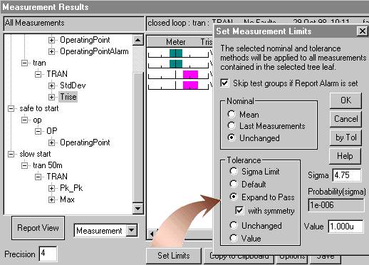
You can set the measurement test limits by expanding the measurements
to "pass with symmetry" in the Results dialog; as shown
below.

If the result is linearly proportional
to the change in the parameter value, then the RSS result is
proportional to the standard deviation which we could obtain
from a statistical analysis. As a matter of convention, each
tolerance is taken as the 3 sigma value, or 3 standard deviations
and we report the RSS results as though they were also 3 sigma.
The parameter perturbation is set to 1 sigma, a compromise between
a negligibly small value and the entire tolerance band. Making
the perturbation fairly large eliminates some errors due to local
maximum values occurring nearby. You can change this variation
by editing the RSS Simulation Template.
For many circuits, the variation of
a measurement with respect to some parameters is highly nonlinear
so that this analysis will give incorrect results, frequently
reporting smaller measurement variations than would be found
using a statistical analysis.
When performing an AC analysis, it is frequently
assumed that the response at each frequency can be considered
independently. Unfortunately, this is a poor assumption because
single frequency results have an ambiguity in phase. When the
difference in phase between 2 simulations is taken, there can
be dramatically different results if one analysis is in a different
phase plane than the reference simulation. Because of this, it
is necessary to phase extend
the vectors we wish to measure. This makes the AC analysis
similar to the transient analysis, requiring measurements that
resolve to scalar values. The duality between frequency and time
seen using the Fourier transform should make this obvious.